# List available example files
list_example_data()climat_example.csv['climat_example.csv']The overall goal of SurEau Climate is to generate hourly forcings from daily climatic variables
 Input: climate_df (DataFrame with daily records),
          date string (DD/MM/YYYY)
                         │
                         ▼
    ┌────────────────────────────────────────────┐
    │  new_climate_day(climate_df, date)         │
    │                                            │
    │  1. Parse date string → DOY, year          │
    │     (dateutil.parser handles any format)   │
    │                                            │
    │  2. Slice row where DATE == date           │
    │                                            │
    │  3. Assign met fields:                     │
    │     T_mean, T_min, T_max                   │
    │     RH_mean, RH_min, RH_max                │
    │     PPT, RG, WS_mean                       │
    │                                            │
    │  4. VPD = f(RH_mean, T_mean)               │
    │                                            │
    │                                            │
    │  5. Look up prev/next row by integer pos   │
    │     → T_min_prev, T_max_prev, T_min_next   │
    │     (needed for diurnal T model)           │
    └────────────────────────────────────────────┘
                          │
                          ▼
                 SurEauClimate object
    ┌────────────────────────────────────────────┐
    │  compute_Rn_and_ETP(clim, params, opts)    │
    │                                            │
    │  Branch: opts.Rn_formulation               │
    │  ─────────────────────────────             │
    │  "Linacre":                                │
    │    nN = 0.25 if PPT > 0 else 0.75          │
    │    (cloud proxy: rainy=cloudy, dry=clear)  │
    │                                            │
    │    SW_abs = (1 − 0.17) × RG × 10⁶          │
    │    LW_loss = 1927.987 × (1+4·nN)           │
    │             × (100 − T_mean)               │
    │                                            │
    │    Rn = max(0,  SW_abs − LW_loss ) × 10⁻⁶  │
    │                                            │
    │  ETP_formulation                           │
    │  ─────────────────────────────             │
    │  "PT": Priestley-Taylor                    │
    │    ETP = α × Δ·Rn / [λ(Δ+γ)]               │
    │    via pyet.priestley_taylor()             │
    │    (α = params.PT_coeff ≈ 1.14)            │
    │                                            │
    │  "PM": Penman-Monteith                     │
    │    es = pyet.calc_es(T)                    │
    │    ea = es − VPD                           │
    │    ETP = pyet.pm(T, WS, Rn, ea, elev)      │
    └────────────────────────────────────────────┘
                         │
                         ▼
            clim.net_radiation, clim.ETP set
    ┌────────────────────────────────────────────┐
    │ new_climate_hourly(clim, opts, veg_params) │
    │                                            │
    │  1. Daylength & solar geometry             │
    │     sunrise_h, sunset_h, daylen_h          │
    │     = daylength(opts.latitude, clim.DOY)   │
    │     Polar edge cases clamped to [0, 24]    │
    │                                            │
    │  2. Radiation disaggregation               │
    │     time_rel = hour × 3600 − sunrise_s     │
    │     io = π/daylen × sin(π·t_rel/daylen)    │
    │     io = 0 outside [sunrise, sunset]       │
    │     RG_h  = RG  × io × 3600  [MJ m⁻² h⁻¹]  │
    │     Rn_h  = Rn  × io × 3600                │
    │                                            │
    │  3. PAR                                    │
    │     PAR_h = PPFD(Watt(RG_h))               │
    │     pot_PAR_h = potential_PAR(h, lat, DOY) │
    │                                            │
    │  4. Temperature disaggregation             │
    │     Parton & Logan model per hour:         │
    │     • Daytime: sine ramp Tmin → Tmax       │
    │     • Evening: exp decay → T_min_next      │
    │     Uses T_min_prev, T_max_prev,           │
    │          T_min_next from adjacent days     │
    │                                            │
    │  5. Relative humidity disaggregation       │
    │     Dewpoint ≈ Tmin (RH_max at sunrise)    │
    │     ea = RH_max/100 × es(Tmin)             │
    │     RH_h = ea / es(T_h) × 100              │
    │     Clipped to [0.5, 100] %                │
    │                                            │
    │  6. Wind speed                             │
    │     WS_h = WS_mean (constant across hours) │
    │                                            │
    │  7. VPD_h = f(RH_h, T_h) per hour          │
    │                                            │
    │  8. ETP disaggregation                     │
    │     "PT": pyet.priestley_taylor(           │
    │              T_h, Rn_h, α, elev)           │
    │     "PM": pyet.pm(T_h, WS_h, Rn_h,         │
    │              ea_h, elev)                   │
    │                                            │
    │  9. Time-step duration n_h                 │
    │     n_h[0]   = ts[0] + (24 − ts[-1])       │
    │     n_h[i>0] = ts[i] − ts[i-1]             │
    │                                            │
    │  10. Subset to opts.time_steps             │
    │      (full 24 h or custom sub-hourly idx)  │
    │                                            │
    │  11. PPT assigned to first time step only  │
    └────────────────────────────────────────────┘
                          │
                          ▼
                 SurEauClimateHourly
                     object (ch)

                          │
                ┌─────────┴──────────┐
                │ Two parallel uses: │
                ▼                    ▼
    ┌───────────────┐  ┌──────────────────────────────────────┐
    │ get_hourly_   │  │  interpolate_climate_hourly(         │
    │ snapshot(     │  │      ch1_arrays, ch2_arrays, p=0.5)  │
    │   ch, idx)    │  │                                      │
    │               │  │  Linear blend between two snapshots: │
    │  Extracts one │  │  field = (1−p)·ch1[f] + p·ch2[f]     │
    │  timestep as  │  │                                      │
    │  a plain dict │  │  Interpolated fields:                │
    │  for passing  │  │  T_air_mean, RG, WS, VPD,            │
    │  into the     │  │  RH_air_mean, ETP, ETP_veg*          │
    │  hydraulic    │  │  (*if present in both snapshots)     │
    │  solver       │  │                                      │
    │               │  │  Non-interpolated fields copied      │
    │  Keys:        │  │  verbatim from ch1                   │
    │  T, RG, WS,   │  │                                      │
    │  VPD, RH,     │  │  Used to refine forcing between      │
    │  ETP, PAR,    │  │  two stored hourly time steps        │
    │  pot_PAR,     │  └──────────────────────────────────────┘
    │  n_hours,     │
    │  time         │
    └───────────────┘
                      │
                      ▼
       Returns:
       • new_climate_day()            → SurEauClimate object
       • compute_Rn_and_ETP()         → SurEauClimate object (Rn + ETP added)
       • new_climate_hourly()         → SurEauClimateHourly object
                                        (RG, Rn, PAR, T, RH, WS, VPD, ETP,
                                         time, n_hours, PPT arrays)
       • get_hourly_snapshot()        → dict (single timestep)
       • interpolate_climate_hourly() → dict (blended between two snapshots)
def new_climate_day(
    climate_df:DataFrame, date:int
)->SurEauClimate:
Extract daily climate from each row of a DataFrame
The column names in the data frame MUST be named as the following:
def compute_Rn_and_ETP(
    clim:SurEauClimate, params:SurEauVegetationParams, opts:SurEauModelOptions
)->SurEauClimate:
Compute daily net radiation and PET.
Given today’s solar radiation, precipitation, and temperature — how much energy is available at the surface, and how much water could potentially evaporate?”
Both outputs are stored back into clim and returned for use in the rest of the model.
Physics notes:
-Rn: Linacre (1968) formulation: shortwave absorbed = (1 - 0.17) × RG longwave loss = 1927.987 × (1 + 4·nN) × (100 - T_mean) nN = 0.25 if PPT > 0 else 0.75
-ETP: Priestley-Taylor: ETP = α × Δ·Rn / λ(Δ+γ)
def new_climate_hourly(
    clim:SurEauClimate, opts:SurEauModelOptions, veg_params:SurEauVegetationParams
)->SurEauClimateHourly:
Disaggregate daily climate to sub-daily time steps.
def interpolate_climate_hourly(
    ch1_arrays:dict, ch2_arrays:dict, p:float=0.5
)->dict:
Linearly interpolate between two hourly climate snapshots.
def get_hourly_snapshot(
    ch:SurEauClimateHourly, idx:int
)->dict:
Extract a single timestep from ClimateHourly as a dict.
# List available example files
list_example_data()climat_example.csv['climat_example.csv']from itables import to_html_datatable
from IPython.display import HTML, display# Load example data
climate_df = load_example_data("climat_example.csv", sep=";")
html_str = to_html_datatable(climate_df)
display(HTML(html_str))| Loading ITables v2.7.3 from the internet... (need help?) |
# Convert numeric columns (all except DATE)
for each_col in climate_df.columns:
    if each_col != "DATE":
climate_df[each_col] = pd.to_numeric(climate_df[each_col], errors="coerce")# Model options
opts = SurEauModelOptions(
# ° N (site location — adjust to your site)
latitude=43.6,
# ← metres above sea level
# SurEauModelOptions.elevation
# elevation = 150,
# ° E
longitude=3.8,
# net radiation model: "Linacre" (only option currently)
Rn_formulation="Linacre",
# PET model: "PT" (Priestley-Taylor) or "PM" (Penman-Monteith)
ETP_formulation="PT",
# True → forces a fixed doy=116 (sunny day template)
constant_climate=False,
# which hours to output (0–23 → full day)
time_steps=np.arange(24),
)# Vegetation parameters
veg_params = SurEauVegetationParams(
# Priestley-Taylor α. Standard = 1.26; tropical humid ≈ 1.1–1.3
PT_coeff=1.14,
)target_date = "01/06/1990" # ← change to any date in the CSV
clim = new_climate_day(climate_df, target_date)clim = compute_Rn_and_ETP(clim, veg_params, opts)
print(f"\n Net radiation (Rn) : {clim.net_radiation:.4f} MJ m⁻² day⁻¹")
print(f" PET (ETP) : {clim.ETP:.4f} mm day⁻¹")
  Net radiation (Rn)  : 22.8024 MJ m⁻² day⁻¹
PET (ETP) : 6.7291 mm day⁻¹hourly_ch = new_climate_hourly(clim, opts, veg_params)print(f"\n Output arrays (24 h each):")
print(
f" ch.T_air_mean [°C] : {hourly_ch.T_air_mean.min():.1f} – {hourly_ch.T_air_mean.max():.1f}"
)
print(
f" ch.RH_air_mean [%] : {hourly_ch.RH_air_mean.min():.1f} – {hourly_ch.RH_air_mean.max():.1f}"
)
print(
f" ch.RG [MJ m⁻² h⁻¹]: {hourly_ch.RG.min():.3f} – {hourly_ch.RG.max():.3f}"
)
print(
f" ch.Rn [MJ m⁻² h⁻¹]: {hourly_ch.Rn.min():.3f} – {hourly_ch.Rn.max():.3f}"
)
print(
f" ch.VPD [kPa] : {hourly_ch.VPD.min():.3f} – {hourly_ch.VPD.max():.3f}"
)
print(
f" ch.ETP [mm h⁻¹] : {hourly_ch.ETP.min():.4f} – {hourly_ch.ETP.max():.4f}"
)
print(
f" ch.PAR [µmol m⁻² s⁻¹]: {hourly_ch.PAR.min():.0f} – {hourly_ch.PAR.max():.0f}"
)
  Output arrays (24 h each):
    ch.T_air_mean  [°C]         : 7.5 – 25.1
    ch.RH_air_mean [%]          : 29.6 – 94.2
    ch.RG          [MJ m⁻² h⁻¹]: 0.000 – 4.791
    ch.Rn          [MJ m⁻² h⁻¹]: 0.000 – 3.867
    ch.VPD         [kPa]        : 0.060 – 2.245
    ch.ETP         [mm h⁻¹]     : 0.0000 – 1.2852
ch.PAR [µmol m⁻² s⁻¹]: 0 – 3061# solar noon
hour = 12
snap = get_hourly_snapshot(hourly_ch, hour)
print(f"\n Snapshot at hour {hour}:00")
for each_param, each_value in snap.items():
print(f" {each_param:<18} : {each_value:.4f}")
  Snapshot at hour 12:00
    T_air_mean         : 22.7493
    RG                 : 4.7912
    WS                 : 1.7000
    VPD                : 1.7082
    RH_air_mean        : 38.3042
    ETP                : 1.2852
    PAR                : 3061.0603
    potential_PAR      : 687.4135
    n_hours            : 1.0000
time : 12.0000week_dates = climate_df["DATE"].iloc[:7].tolist()
daily_summary = []
for date in week_dates:
c = new_climate_day(climate_df, date)
c = compute_Rn_and_ETP(c, veg_params, opts)
h = new_climate_hourly(c, opts, veg_params)
daily_summary.append(
{
"date": date,
"Rn": c.net_radiation,
"ETP": c.ETP,
"T_mean": c.T_air_mean,
"VPD": c.VPD,
"ETP_sum_hourly": float(np.nansum(h.ETP)),
}
)
print(
f"\n {'Date':<12} {'Rn':>8} {'ETP_day':>9} {'ETP_Σh':>8} {'T_mean':>8} {'VPD':>8}"
)
print(f" {'':12} {'MJ/m²':>8} {'mm/d':>9} {'mm/d':>8} {'°C':>8} {'kPa':>8}")
print(" " + "-" * 57)
for each_row in daily_summary:
print(
f" {each_row['date']:<12} {each_row['Rn']:8.3f} {each_row['ETP']:9.4f} "
f"{each_row['ETP_sum_hourly']:8.4f} {each_row['T_mean']:8.2f} {each_row['VPD']:8.4f}"
)
  Date               Rn   ETP_day   ETP_Σh   T_mean      VPD
                  MJ/m²      mm/d     mm/d       °C      kPa
  ---------------------------------------------------------
  01/01/1990      0.822    0.1300   0.1333    -3.25   0.0148
  02/01/1990      1.886    0.3155   0.3242    -1.95   0.0163
  03/01/1990      0.078    0.0138   0.0141    -0.70   0.0179
  04/01/1990      0.157    0.0272   0.0276    -1.20   0.0173
  05/01/1990      0.565    0.1066   0.1092     1.05   0.0228
  06/01/1990      0.420    0.0829   0.0845     2.25   0.0222
07/01/1990 0.375 0.0680 0.0688 0.05 0.0189HOURS = np.arange(24)
COLORS = {
"T": "#e74c3c",
"RH": "#3498db",
"Rg": "#f39c12",
"VPD": "#9b59b6",
"ETP": "#27ae60",
"PAR": "#e67e22",
}fig1, axes = plt.subplots(3, 2, figsize=(13, 10), sharex=True)
fig1.suptitle(
f"Hourly Climate Forcings — {target_date} (DOY {clim.DOY})\n"
f"Site: {opts.latitude}°N, {opts.longitude}°E | Rn: {clim.net_radiation:.3f} MJ m⁻² | "
f"ETP: {clim.ETP:.3f} mm d⁻¹",
fontsize=12,
fontweight="bold",
)
panels = [
(axes[0, 0], hourly_ch.T_air_mean, "Temperature (°C)", COLORS["T"], None),
(axes[0, 1], hourly_ch.RH_air_mean, "Relative Humidity (%)", COLORS["RH"], None),
(axes[1, 0], hourly_ch.RG, "Solar Radiation (MJ m⁻² h⁻¹)", COLORS["Rg"], None),
(axes[1, 1], hourly_ch.VPD, "VPD (kPa)", COLORS["VPD"], None),
(axes[2, 0], hourly_ch.ETP * 1000, "ETP (×10⁻³ mm h⁻¹)", COLORS["ETP"], None),
(
axes[2, 1],
hourly_ch.PAR,
"PAR (µmol m⁻² s⁻¹)",
COLORS["PAR"],
hourly_ch.potential_PAR,
),
]
for ax, y, ylabel, color, y2 in panels:
ax.fill_between(HOURS, y, alpha=0.18, color=color)
ax.plot(HOURS, y, color=color, lw=2)
if y2 is not None:
ax.plot(HOURS, y2, color="gray", lw=1.2, ls="--", label="Potential PAR")
ax.legend(fontsize=8)
ax.set_ylabel(ylabel, fontsize=9)
ax.set_xlim(0, 23)
ax.grid(True, alpha=0.25, ls=":")
ax.axvspan(0, clim.DOY and 6, alpha=0.05, color="navy") # night shading
ax.axvspan(20, 23, alpha=0.05, color="navy")
for ax in axes[2, :]:
ax.set_xlabel("Hour of day", fontsize=9)
ax.set_xticks(range(0, 24, 3))
plt.tight_layout()
plt.show()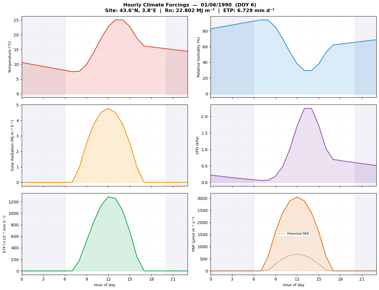
n_days = len(week_dates)
fig2, axes2 = plt.subplots(2, 1, figsize=(13, 7), sharex=True)
fig2.suptitle(
    "Week of Hourly Forcings — Temperature & ETP", fontsize=12, fontweight="bold"
)

all_T = []
all_ETP = []
all_VPD = []
all_RG = []
x_ticks = []
x_labels = []

for i, date in enumerate(week_dates):
    c = new_climate_day(climate_df, date)
    c = compute_Rn_and_ETP(c, veg_params, opts)
    h = new_climate_hourly(c, opts, veg_params)
    offset = i * 24
    x = np.arange(offset, offset + 24)
    all_T.extend(h.T_air_mean)
    all_ETP.extend(h.ETP)
    all_RG.extend(h.RG)
    all_VPD.extend(h.VPD)
    x_ticks.append(offset + 12)
    x_labels.append(date)

X = np.arange(len(all_T))

ax = axes2[0]
ax.fill_between(X, all_T, alpha=0.25, color=COLORS["T"])
ax.plot(X, all_T, color=COLORS["T"], lw=1.5, label="Temperature")
ax2r = ax.twinx()
ax2r.fill_between(X, all_RG, alpha=0.15, color=COLORS["Rg"])
ax2r.plot(X, all_RG, color=COLORS["Rg"], lw=1.2, label="Solar Rad.")
ax.set_ylabel("Temperature (°C)", color=COLORS["T"], fontsize=9)
ax2r.set_ylabel("RG (MJ m⁻² h⁻¹)", color=COLORS["Rg"], fontsize=9)
ax.grid(True, alpha=0.2, ls=":")
for d in range(n_days):
    ax.axvline(d * 24, color="gray", lw=0.5, ls="--")

ax = axes2[1]
ax.fill_between(X, [e * 1000 for e in all_ETP], alpha=0.25, color=COLORS["ETP"])
ax.plot(X, [e * 1000 for e in all_ETP], color=COLORS["ETP"], lw=1.5, label="ETP")
ax2r2 = ax.twinx()
ax2r2.fill_between(X, all_VPD, alpha=0.15, color=COLORS["VPD"])
ax2r2.plot(X, all_VPD, color=COLORS["VPD"], lw=1.2, label="VPD")
ax.set_ylabel("ETP (×10⁻³ mm h⁻¹)", color=COLORS["ETP"], fontsize=9)
ax2r2.set_ylabel("VPD (kPa)", color=COLORS["VPD"], fontsize=9)
ax.set_xlabel("Day", fontsize=9)
ax.set_xticks(x_ticks)
ax.set_xticklabels(x_labels, rotation=30, ha="right", fontsize=8)
ax.grid(True, alpha=0.2, ls=":")
for d in range(n_days):
    ax.axvline(d * 24, color="gray", lw=0.5, ls="--")

plt.tight_layout()
plt.show()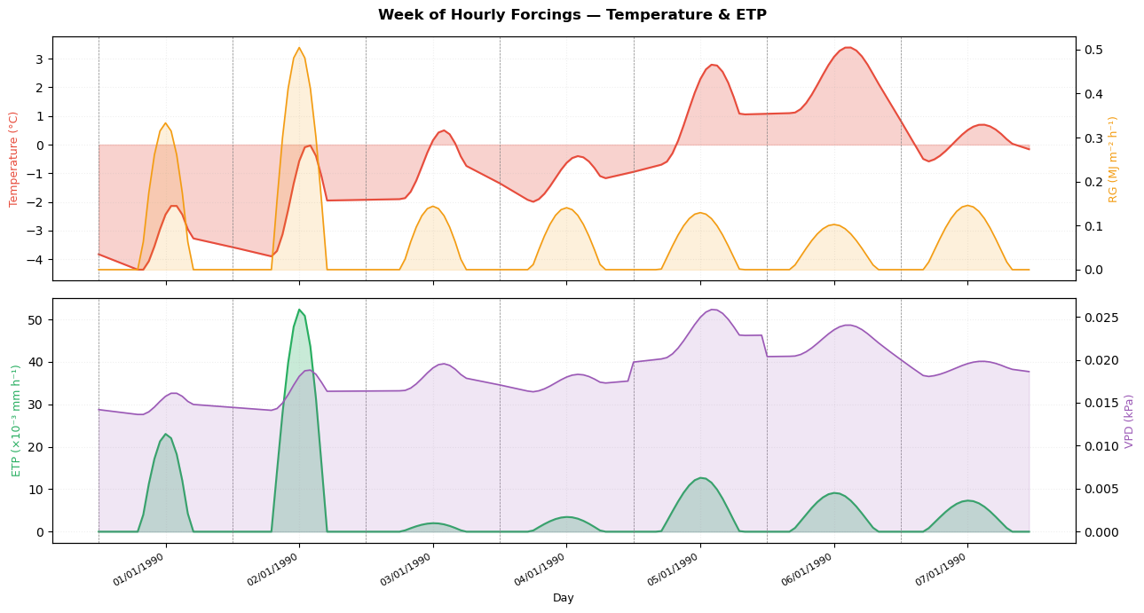
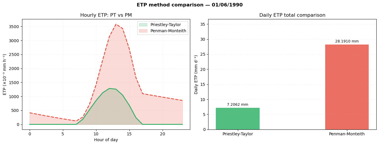
fig3, axes3 = plt.subplots(1, 2, figsize=(13, 5))
fig3.suptitle(f"ETP method comparison — {target_date}", fontsize=12, fontweight="bold")

# PT
opts_pt = SurEauModelOptions(**{**vars(opts), "ETP_formulation": "PT"})
c_pt = new_climate_day(climate_df, target_date)
c_pt = compute_Rn_and_ETP(c_pt, veg_params, opts_pt)
h_pt = new_climate_hourly(c_pt, opts_pt, veg_params)

# PM
opts_pm = SurEauModelOptions(**{**vars(opts), "ETP_formulation": "PM"})
c_pm = new_climate_day(climate_df, target_date)
c_pm = compute_Rn_and_ETP(c_pm, veg_params, opts_pm)
h_pm = new_climate_hourly(c_pm, opts_pm, veg_params)

ax = axes3[0]
ax.fill_between(
    HOURS, h_pt.ETP * 1000, alpha=0.2, color=COLORS["ETP"], label="Priestley-Taylor"
)
ax.plot(HOURS, h_pt.ETP * 1000, color=COLORS["ETP"], lw=2)
ax.fill_between(
    HOURS, h_pm.ETP * 1000, alpha=0.2, color="#e74c3c", label="Penman-Monteith"
)
ax.plot(HOURS, h_pm.ETP * 1000, color="#e74c3c", lw=2, ls="--")
ax.set_xlabel("Hour of day")
ax.set_ylabel("ETP (×10⁻³ mm h⁻¹)")
ax.set_title("Hourly ETP: PT vs PM")
ax.legend()
ax.grid(True, alpha=0.25, ls=":")

# Bar comparison daily totals
ax2 = axes3[1]
methods = ["Priestley-Taylor", "Penman-Monteith"]
daily_totals = [float(np.nansum(h_pt.ETP)), float(np.nansum(h_pm.ETP))]
bars = ax2.bar(
    methods, daily_totals, color=[COLORS["ETP"], "#e74c3c"], alpha=0.8, width=0.4
)
ax2.bar_label(bars, fmt="%.4f mm", padding=3, fontsize=9)
ax2.set_ylabel("Daily ETP (mm d⁻¹)")
ax2.set_title("Daily ETP total comparison")
ax2.set_ylim(0, max(daily_totals) * 1.3)
ax2.grid(True, alpha=0.25, ls=":", axis="y")

plt.tight_layout()
plt.show
ETP_formulation is PM
Remember to adjust the lat/lon